Research

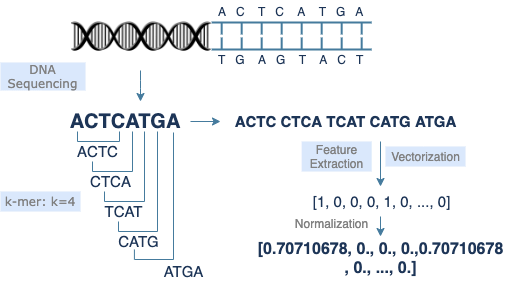
My research is motivated by the expansion of “big data” and the challenges introduced in these high-dimensional settings. A prominent example arises in genomics, where researchers analyze large biological datasets to understand how genetic variation influences traits and disease. In such research, DNA is extracted and sequenced, producing tens of thousands of features, each representing a gene, nucleotide, or molecular marker.

Source: Medium — Xiaofan Luan

Reducing this immense dimensionality of features to capture the essential biological signal is critical for revealing meaningful genetic structure, improving disease prediction, and developing targeted therapies. My research addresses these issues by developing sufficient dimension reduction methodologies that extract the most informative structures from high-dimensional data and project them onto lower-dimensional subspaces for improved modeling, inference, and visualization.

Sufficient Dimension Reduction

Basics

Dimension reduction is often associated with the field of multivariate statistics, which is a field that can carry a reputation for being difficult due to its heavy use of matrix algebra and abstract geometric concepts. While this perception has some truth—even for me, as I often have to revisit the underlying math—dimension reduction is actually quite intuitive and something people constantly do without realizing it. In fact, this paragraph is a form of dimension reduction. That is, dimension reduction is simply the act of reducing the size of any information into a smaller and more digestible form. Ever skip through a video just to catch the main points or watch a TikTok at 2x speed? Both are examples of dimension reduction, with countless more found in everyday life. However, sometimes when watching a video at 2x speed, you may miss important details, and a slightly slower speed would be better. This illustrates the idea of sufficient dimension reduction (SDR), which is the process of reducing data to its smallest possible form while still preserving all the essential information relevant to the question or goal of interest.

Formal Definition & Central Subspace

In mathematical terms, let $Y$ represent the response or variable of interest that we want to preserve, and let $\mathbf{X} \in \mathbb{R}^{p}$ represent the predictor or data we have with $p$ features. Then, the goal of SDR is to project $\mathbf{X}$ onto the smallest possible subspace $\mathcal{S} \subseteq \mathbb{R}^{p}$ without any loss of information with respect to $Y \mid \mathbf{X}$, which denotes the conditional distribution of $Y$ given $\mathbf{X}$ . So how do we get this smallest possible subspace? Cook (1998) introduced the central subspace $\mathcal{S}_{Y \mid \mathbf{X}}$, which is the intersection of all possible dimension reduction subspaces. Thus, $\mathcal{S}_{Y \mid \mathbf{X}}$ is the unique and minimal dimension reduction subspace that preserves all the information about $Y$ given $\mathbf{X}$. Therefore, most SDR methods developed are trying to estimate $\mathcal{S}_{Y \mid \mathbf{X}}$. Let $d < p$ be the dimension of $\mathcal{S}_{Y \mid \mathbf{X}}$ and $\boldsymbol{\beta} = \left(\boldsymbol{\beta}_{1}, \ldots, \boldsymbol{\beta}_{d}\right)$ be a basis matrix of $\mathcal{S}_{Y\mid \mathbf{X}}$ determined by the particular SDR technique. Then, SDR methods can reduce the dimensionality of the features to $\boldsymbol{\beta}^{\top}\mathbf{X} \in \mathbb{R}^{d}$ for subsequent supervised learning without loss of information.

Eigenvectors for Dimension Reduction

So, how do we determine the projection matrix $\boldsymbol{\beta} \in \mathbb{R}^{p \times d}$ used in SDR to reduce the data from $p$ dimensions to $d < p$ dimensions? Most SDR methods determine $\boldsymbol{\beta}$ by using eigenvectors (if you already understand eigenvectors, feel free to skip below). Suppose we have data given by the matrix $\mathbf{A} \in \mathbb{R}^{p \times p}$, then eigenvectors are any vector $\mathbf{v} \in \mathbb{R}^{p}$ that satisfy $\mathbf{A}\mathbf{v} = \lambda \mathbf{v}$, where $\lambda$ is a scaler value. Most encounter this concept in a linear algebra course and learn how to numerically solve for $\mathbf{v}$. However, I find it is not always clear to most what an eigenvector represents beyond its formulation, or at least for me it initially wasn’t. So, I’ll try my best to give a visual representation that makes the idea more intuitive. As a reminder, in dimension reduction we aim to transform our data into a smaller form. Thus, if we think about our data matrix $\mathbf{A}$ and an arbitrary vector $\boldsymbol{\omega}$, multiplying $\mathbf{A} \boldsymbol{\omega}$ applies a linear transformation that can rotate, stretch, or compress the data in space. We show this transformation below for a typical vector $\boldsymbol{\omega}$ and an eigenvector $\mathbf{v}$.

A typical vector ($\mathbf{\omega}$)

An eigenvector ($\mathbf{v}$)

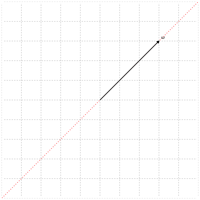
In the figures above, the grid represents the transformation, and the dotted line (red) shows all possible points that lie along the same direction as the vector, i.e., the span of the vector. We see that the typical vector $\boldsymbol{\omega}$ is knocked off its span after the transformation, which means its direction changes and it no longer preserves the same information in the data. In contrast, the eigenvector $\mathbf{v}$ only stretches slightly. The amount by which the eigenvector stretches is its eigenvalue $\lambda$. Hence, the eigenvector $\mathbf{v}$ stays on its span during the transformation and thereby represents a principal direction of the data matrix $\mathbf{A}$. If we find all the eigenvectors of $\mathbf{A}$, they form the coordinate system aligned with how $\mathbf{A}$ transforms space. Therefore, by using $d$ of the eigenvectors to form the basis for the projection matrix, we can reduce the data onto these principal directions and effectively capture the dominant structure of $\mathbf{A}$ in a lower $d$-dimensional space.

Generalized Eigenvalue Problem

Most SDR methods do not simply use the eigenvectors of the data matrix $\mathbf{X}$ to construct the projection matrix $\boldsymbol{\beta}$. Why? Because doing so still involves the entire dataset, which can be extremely large, computationally expensive, and contain a lot of noise. Instead, it is often more practical to work with summary measures of the data, such as means and covariances. Moreover, in SDR we are specifically concerned with preserving all information in the response $Y$ with respect to the predictor $\mathbf{X}$. Thus, most SDR methods construct a method-specific kernel matrix $\mathbf{M} \in \mathbb{R}^{p \times p}$ that captures the relationship between $Y$ and $\mathbf{X}$. For example, Li (1991) introduced this concept through the sliced inverse regression (SIR) method by proposing the kernel matrix $\mathbf{M}_{SIR} = \text{Cov}\left(\mathbb{E}[\mathbf{X} - \mathbb{E}(\mathbf{X}|Y)]\right)$. Li (2007) then showed that most SDR methods are formulated by solving the generalized eigenvalue problem

where $\mathbf{N} \in \mathbb{R}^{p \times p}$ is a symmetric and positive definite matrix often taken to be the covariance matrix of $\mathbf{X}$, denoted $\boldsymbol{\Sigma}_{\mathbf{X}}$.

Dimension Reduction Subspace Criteria

Once the kernel matrix $\mathbf{M}$ used in the generalized eigenvalue problem and the optimal dimension $d$ to which the data should be reduced have been determined, researchers have traditionally used the $d$ eigenvectors corresponding to the largest eigenvalues to construct the basis for the projection matrix $\boldsymbol{\beta}$. Let $\mathbf{v}_{1}, \ldots, \mathbf{v}_{p}$ be the eigenvectors corresponding to the eigenvalues $\lambda_{1} \geq \ldots \geq \lambda_{p}$. Then, traditionally, $(\mathbf{v}_{1}, \ldots, \mathbf{v}_{d}) \in \mathbb{R}^{p \times d}$ is used as the projection matrix $\boldsymbol{\beta}$. Most work in SDR focuses on proposing new ways to construct $\mathbf{M}$ or developing methods to determine $d$. While my research explores these directions, a central contribution of my work is the introduction of the field of dimension reduction subspace ordering criteria, which directly questions the long-standing use of eigenvalues as the criterion for selecting the eigenvectors used to construct the projection matrix.

Eigenvalues generally represent the variability of the data in their respective eigenvector subspaces. Hence, by choosing the eigenvectors corresponding to the largest eigenvalues, the idea is that these selected eigenvectors maximize the variability of the data in the resulting lower-dimensional subspace. However, eigenvalues are a flawed criterion because maximizing variability does not guarantee that the selected subspace preserves the relationship between the response and predictors, which is the goal of SDR. Thus, in Boonstra et al. (2025), we propose new subspace ordering criteria that explicitly capture the predictive information in each subspace to ensure that the selected subspaces align with the intended goal of the supervised learner.

Binary Response

To illustrate this, consider a simple example with two populations whose respective mean vectors are $\boldsymbol{\mu}_{1} = (0, 0, 0)$ and $\boldsymbol{\mu}_{2} = (0, 0, \alpha)$. Additionally, let both populations share the common covariance matrix \(\boldsymbol{\Sigma} = \begin{bmatrix} 3 & 0 & 0 \\ 0 & 2 & 0 \\ 0 & 0 & 1 \end{bmatrix}.\) Consider the most popular SDR technique, principal components, in which dimension reduction is defined by the eigenvectors of $\boldsymbol{\Sigma}$. It is easily shown that the eigenvectors of $\boldsymbol{\Sigma}$ are $\mathbf{v}_1 = (1, 0, 0)^\top$, $\mathbf{v}_2 = (0, 1, 0)^\top$, and $\mathbf{v}_3 = (0, 0, 1)^\top$, with respective eigenvalues $\lambda_1 = 3$, $\lambda_2 = 2$, and $\lambda_3 = 1$. Thus, since $\lambda_{1} > \lambda_{2} > \lambda_{3}$, the dimension reduction subspace is traditionally taken to be $(\mathbf{v}_{1}, \mathbf{v}_{2}, \mathbf{v}_{3})$. Moreover, since there are two populations with a common covariance matrix, the optimal dimension to reduce to is $d = 1$, and as a result, $\mathbf{v}_1$ would be chosen as the projection vector and most informative subspace based on the eigenvalues. However, from the figure below, we clearly see this is not true.

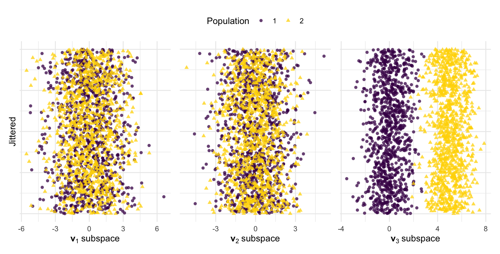
To generate the figure, we simulated data and plotted the data in each eigenvector subspace. The goal is for the populations to remain distinct and separated in the reduced subspaces. However, only $\mathbf{v}_{3}$, the eigenvector corresponding to the smallest eigenvalue, preserves the differences between the populations. The reason for this is clear. The only difference between the populations was due to $\alpha$ in $\boldsymbol{\mu}_{2}$, which affected the third feature. Thus, only $\mathbf{v}_3 = (0, 0, 1)^\top$ captures this difference. Motivated by this, we proposed a criterion that correctly identifies $\mathbf{v}_{3}$ as the most informative subspace. Specifically, we proposed a population signal-to-noise ratio given by

which is the population analogue of the independent Student’s T-statistic. For our example, $\Delta_{1} = 0$, $\Delta_{2} = 0$, and $\Delta_{3} = \alpha$. Thus, since $\Delta_{3} > \Delta_{2} = \Delta_{1}$, the eigenvectors should be reordered by their importance as $(\mathbf{v}_{3}, \mathbf{v}_{2}, \mathbf{v}_{1})$. Under the traditional eigenvalue ordering framework, $\mathbf{v}_{3}$ would never have been considered; however, our criterion $\Delta_{j}$ correctly identified $\mathbf{v}_{3}$ as the most informative subspace. See Boonstra et al. (2025) for additional details and theoretical results.

Categorical or Continuous Response

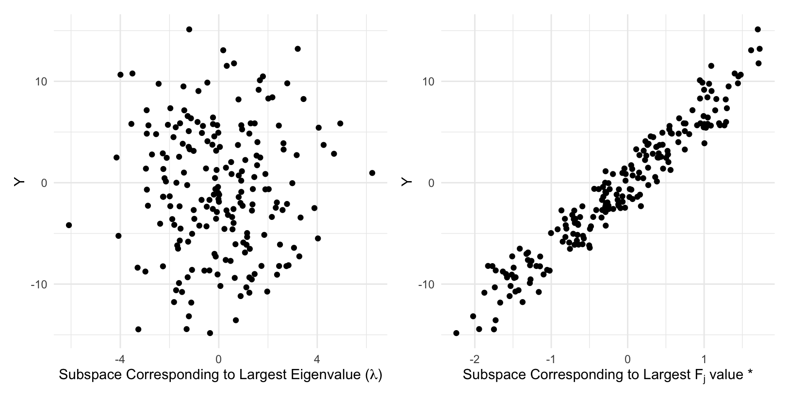
In Boonstra et al. (2025), we naturally extend the idea of subspace ordering criteria to a categorical response with more than two populations by using an F-statistic, denoted as $F_{j}$. When a response is continuous, most SDR methods discretize the response Y into H contiguous non-overlapping intervals called slices to estimate conditional moments for constructing $\mathbf{M}$. Similarly, by treating the $H$ slices as categories, we can apply the $F_{j}$ criterion when the response is continuous to maximize slice separation, which often identifies subspaces that best capture the conditional moments. An example for multiple SDR methods is shown below using simulated data with $Y_{i} = \boldsymbol{\beta}^{\top}\mathbf{X}_{i} + \varepsilon_{i},$ where $\boldsymbol{\beta} \in \mathbb{R}^{p}$ has i.i.d. entries from a $\mathcal{N}(0, 1)$ distribution and $\varepsilon_{i}$ follows a $\mathcal{N}(0, 1)$ distribution. We can clearly see that using the $F_{j}$ criterion instead of eigenvalues identifies subspaces that best preserve the relationship between the response and the predictors.

Publications & Manuscripts

Boonstra, D. T., Kim, R., and Young, D. M. (2025).
“Subspace Ordering for Maximum Response Preservation in Sufficient Dimension Reduction.”
Under Review doi: 10.48550/arXiv.2510.27593 pdf code

Boonstra, D. T., Kim, R., and Young, D. M. (2025).
“Precision Matrix Regularization in Sufficient Dimension Reduction for Improved Quadratic Discriminant Classification.”
Under Review doi: 10.48550/arXiv.2506.19192 pdf code

Manuscripts in Progress

Boonstra, D. T., Kim, R., and Young, D. M.
“Heteroscedastic Invariant Sufficient Dimension Reduction.”

Boonstra, D. T., Kim, R., and Young, D. M.
“Sufficient Dimension Reduction Methods for High-Dimensional Data Are Overly Complicated.”

Boonstra, D. T., Kim, R., and Young, D. M.
“Ordering Dimension Reduction Subspaces via a Quadratic Discriminant Optimal Error Rate.”